I couldn’t miss the fun Twitter hashtag #BadStockPhotosOfMyJob thanks to a tweet by Julia Silge and another one by Colin Fay. The latter inspired me to actually go and look for what makes a data science photo… What characterizes “data science” stock photos?

My (not bad) stock photo source

Pexels metadata for the win

Where to find information related to stock photos? In two previous blog posts of mine I used Pexels, a website providing CC0 pictures which is quite nice. My goal was to obtain the titles and the tags of stock photos of “data science”: for instance if you look at this picture, its tags are “business”, “contemporary”, “computer”, etc. Pexels tags are very useful metadata, saving me the effort to use machine learning methods to analyse images.

Responsible webscraping

When researching this post I discovered that Pexels has an API, documented here but this API does not get you the title nor the tags associated to a picture so only webscraping could get me what I needed.

Webscraping is a powerful tool allowing one to rectangle webpages but with great power comes great responsability. Being able to scrape a webpage does not mean you are allowed to. You could get sued or your IP could get blocked. I am far from being an expert but I often read Bob Rudis’ blog where I learnt about rOpenSci’s robotstxt package that does “robots.txt file parsing and checking for R” which in plain language means it checks for you what a webpage legally allows you to do. See below,

# how I'll find pictures
robotstxt::paths_allowed("https://www.pexels.com/search")

## [1] TRUE

# where tags live
robotstxt::paths_allowed("https://www.pexels.com/photo")

## [1] TRUE

robots.txt files often also tell you how often you can hit a page by defining a “crawling delay”. Sadly Pexels robots.txt doesn’t:

robotstxt::get_robotstxt("https://www.pexels.com")

## Sitemap: https://s3.amazonaws.com/pexels/sitemaps/sitemap.xml.gz

But Bob Rudis, who was patient and nice enough to answer my questions, told me that I should probably respect the rate limit defined in Pexels API docs. “Do not abuse the API. The API is rate-limited to 200 requests per hour and 20,000 requests per month.” As I recently explained in a post on Locke Data’s blog, these days to limit rate of a function I use the very handy ratelimitr package by Tarak Shah.

limited_get <- ratelimitr::limit_rate(httr::GET,
                                      ratelimitr::rate(200, 60*60),# not more than 200 times an hour
                                      ratelimitr::rate(1, 5))#not more than 1 time every 5 seconds

Elegant webscraping

At the time of the two aforelinked blog posts I had used RSelenium to scroll down and get the download link of many pictures, but Bob Rudis wrote an elegant and cool alternative using query parameters, on which I’ll build in this post.

I first re-wrote the function to get all 15 pictures of each page of results.

get_page <- function(num = 1, seed = 1) {
  message(num)
  limited_get(
    url = "https://www.pexels.com/search/data science/",
    query = list(
      page=num,
      seed=seed
    )
  ) -> res
  
  httr::stop_for_status(res)
  
  pg <- httr::content(res)
  
  tibble::tibble(
    url = rvest::html_attr(rvest::html_nodes(pg, xpath = "//a[@class='js-photo-link']"), "href"),
    title = rvest::html_attr(rvest::html_nodes(pg, xpath = "//a[@class='js-photo-link']"), "title"),
    tags = purrr::map(url, get_tags)
  )
  
} 

I re-wrote it because I needed the “href” and because it seems that the structure of each page changed a bit since the day on which the gist was written. To find out I had to write “a[@class='js-photo-link’]” I inspected the source of a page.

Then I wrote a function getting tags for each picture.

get_tags <- function(url){
  message(url)
  url <- paste0("https://www.pexels.com", url)
  res <- limited_get(url)
  httr::stop_for_status(res)
  pg <- httr::content(res)
  nodes <- rvest::html_nodes(pg, xpath = '//a[@data-track-label="tag" ]')
  rvest::html_text(nodes)
}

And finally I got results for 20 pages. I chose 20 without thinking too much. It seemed enough for my needs, and each of these pages had pictures.

ds_stock <- purrr::map_df(1:20, get_page)
ds_stock <- unique(ds_stock)
ds_stock <- tidyr::unnest(ds_stock, tags)

I got 300 unique pictures.

What’s in a data science stock photo?

Now that I have all this information at hand, I can describe data science stock photos!

Data science tags

library("ggplot2")
library("ggalt")
library("hrbrthemes")
tag_counts <- dplyr::count(ds_stock, tags, sort = TRUE)[1:10,]

dplyr::mutate(tag_counts,
              tags = reorder(tags, n)) %>% 
ggplot() +
  geom_lollipop(aes(tags, n),
                size = 2, col = "salmon") +
  hrbrthemes::theme_ipsum(base_size = 16,
                          axis_title_size = 16) +
  xlab("Tag") +
  ggtitle("300 data science stock photos",
          subtitle = "Most frequent tags. Source: https://www.pexels.com") +
  coord_flip()

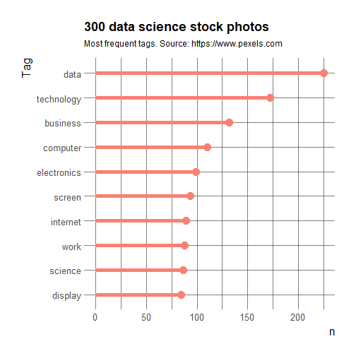
So the most common tags are data, technology, business and computer. Not too surprising!

Data science scenes

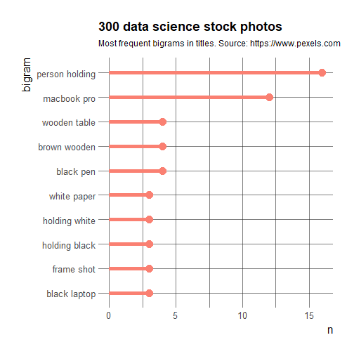
Now, let’s have a look at titles that are in general more descriptive of what’s happening/present on the photo (i.e. is the computer near a cup of coffee or is someone working on it). I tried using a technique described in Julia Silge’s and David Robinson’s Tidy text mining book: “Counting and correlating pairs of words with the widyr package” described in this section of the book but it wasn’t too interesting because most correlation values were too low. One issue was probably my having too few titles: only half of pictures have titles! So I’ll resort to plotting most common bigrams, which I learnt in the Tidy text mining book as well.

stopwords <- rcorpora::corpora("words/stopwords/en")$stopWords

ds_stock %>%
  dplyr::filter(!is.na(title)) %>%
  dplyr::select(title) %>%
  unique() %>%
  tidytext::unnest_tokens(bigram, title,
                          token = "ngrams", n = 2)  %>%
  tidyr::separate(bigram, c("word1", "word2"), sep = " ",
                  remove = FALSE)  %>%
  dplyr::filter(!word1 %in% stopwords) %>%
  dplyr::filter(!word2 %in% stopwords)%>%
  dplyr::count(bigram, sort = TRUE) %>%
  dplyr::mutate(bigram = reorder(bigram, n)) %>%
  head(n = 10)%>%
ggplot() +
  geom_lollipop(aes(bigram, n),
                size = 2, col = "salmon") +
  hrbrthemes::theme_ipsum(base_size = 16,
                          axis_title_size = 16) +
  ggtitle("300 data science stock photos",
          subtitle = "Most frequent bigrams in titles. Source: https://www.pexels.com")+
  coord_flip()

So there’s a lot of holding computer happening, and these laptops are either black or white… And well Macbook Pro probably looks more professional?

Hold my laptop and watch…

my trying to find a good post conclusion! In this post, I tried to responsibly and elegantly scrape rich photo metadata from Pexels to characterize stock photos of data science. Using tags, and most common bigrams in titles, I found that data science stock photos are associated with data, business and computers; and that they often show people holding computers. Now, you’ll excuse me while I try and comfort my poor pink laptop that feels a bit too un-data-sciency.