Our brand-new baby received a fantastic picture book as a gift: Possum magic, a classic for Aussie kids. Thanks, Miles! In that book, Hush the possum and her Grandma Poss encounter different Australian animals and travel across well eat their way through the country. It is an adorable story with great illustrations! Reading it will make you feel like travelling to Australia, for instance to useR! 2018, except you shouldn’t because it is a very scary country:
Rough night with 👶. ☕ was a good start but it was the balcony 🐍 capture and release that really 💓
— Miles McBain (@MilesMcBain) 25 d’agost de 2017
However, you can travel and learn geography without leaving the comfort of a snake-free home… by mapping Hush’s adventures! Which is what I decided to do.
We shall prepare data for the maps in two main steps: first, looking where one can find the animals mentioned in the book; second, attributing a longitude and latitude to the cities Hush goes to.
Locating the animals, snake included
In the book, we first learn about how the magic of Grandma Poss affects some animals: wombats, kookaburras, dingoes and emus. We then read how Hush’s invisibility (sorry, spoiler) makes her interact with koalas, kangaroos and snakes. We can imagine Hush and her grandmother live near these animals, in what is called “deep in the Australian bush”. We’ll map where all these animals live so that we can guess where Hush can live for the story to be credible (I admit that the magic part kind of throws this plan out the window, oh well). Moreover, given what Wikipedia says about the bush, Hush and her grandmother could live anywhere in Australia as long as it’s not in a city, and since Hush’s first city visit is in Adelaide, we can suppose she did not live too far away from there. Let’s see!
In order to map animals, we shall get occurrences from 2011 to 2016 via the rOpenSci spocc package, with GBIF as a data source, and using the scrubr package for cleaning, like in my blog post visualizing waxwings migration. When querying data via spocc one needs a bounding box, so I’ll first load an Australian map from the eechidna package, product from the rOpenSci 2016 Oz unconf. I was inspired by the code in this blog post that’s also a product from an Oz unconf.
library("eechidna")
library("ggthemes")
library("ggplot2")
data(nat_map_2016)
Let’s just draw an empty map.
ozmap <- ggplot() +
                geom_map(aes(map_id=id), data=nat_map_2016,
                         map=nat_map_2016) +
                expand_limits(x=nat_map$long, y=nat_map$lat) +
                theme_map()
ozmap

And now, let’s prepare the bounding box!
bbox <- c(min(nat_map$long), min(nat_map$lat),
          max(nat_map$long), max(nat_map$lat))
I’ll make some assumptions about species and families since the book is not completely clear regarding which animals are meant exactly. Before pondering about this I had no idea there were three species of wombats! For wombats, I’m using the two possible families, for kookaburras, emus and kangaroos the whole family and for snake the one mentioned in that scary thread. For possums, I’m using a family of possums whose Wikipedia page did not indicate they were mostly urban.
animals <- tibble::tibble(name = c("wombat", "wombat", "kookaburra",
                                   "dingo", "emu",
                                   "koala", "kangaroo",
                                   "snake", "possum"),
                          latin = c("Lasiorhinus", "Vombatus", "Dacelo",
                                    "Canis lupus dingo", "Dromaius",
                                    "Phascolarctos cinereus", "Macropus",
                                    "Morelia spilota", "Phalangeridae"))
knitr::kable(animals)
| name | latin |
|---|---|
| wombat | Lasiorhinus |
| wombat | Vombatus |
| kookaburra | Dacelo |
| dingo | Canis lupus dingo |
| emu | Dromaius |
| koala | Phascolarctos cinereus |
| kangaroo | Macropus |
| snake | Morelia spilota |
| possum | Phalangeridae |
Here is the function to get occurrences for one species or family.
library("spocc")
library("scrubr")
library("magrittr")
get_ozccurrences <- function(latin, year, bbox){
  gbifopts <- list(year = year)
  ozccurrences <- occ(query = latin,
                      from = c('gbif'),
                      gbifopts = gbifopts,
                      limit = 200000,
                      geometry = bbox)
  ozccurrences <- occ2df(ozccurrences)
  ozccurrences <- ozccurrences %>%
    coord_impossible() %>%
    coord_incomplete() %>%
    coord_unlikely() %>%
    date_standardize("%Y-%m-%d") %>%
    date_missing()
  ozccurrences$latin <- latin
  ozccurrences
}
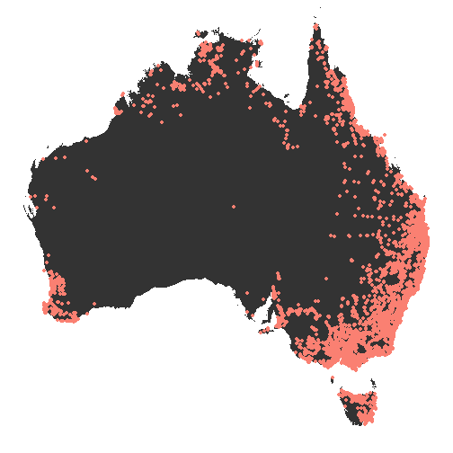
Let’s test it on kookaburras in 2016, using the whole family. Note, the maps drawn in this section are really meant to just have a look. In a better analysis I’d try to define zones based on the occurrences for instance, and I’d be more perfectionist regarding the looks of the map.
kookaburras <- get_ozccurrences("Dacelo", bbox = bbox, year = 2016)

ozmap +
  geom_point(data = kookaburras,
             aes(longitude, latitude),
             col = "salmon")

Note that occurrences might be misleading, since to get one you need one observer, so we’ll probably get less occurrences when there are less humans without this meaning the density of the animal itself is lower. But since Hush’s story is told by a human, we expect Hush to live in an area with at least a few observations of the different animals! Otherwise, how could the author know about all this stuff?
all_ozcurrences <- purrr::map2_df(rep(animals$latin, 6),
                                 rep(2011:2016, nrow(animals)),
                                 get_ozccurrences,
                                 bbox = bbox)
all_ozcurrences <- dplyr::rename(all_ozcurrences, scientific_name = name)
all_ozcurrences <- dplyr::left_join(all_ozcurrences, animals, by = "latin")
readr::write_csv(all_ozcurrences, path = "data/2017-12-15-all_ozcurrences.csv")
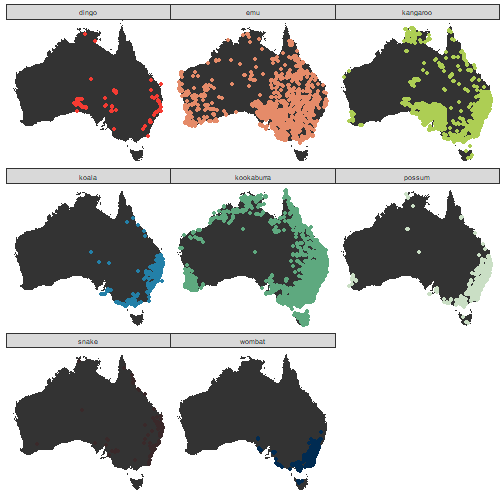
Now that we have a reasonable number of occurrences, we can check where the animals have been seen, hopefully all of them have at least one place in common, preferably not too far from Adelaide (whose location we’ll show in the next section). Although colours are not needed here, I’ll get a bit artistic and use the pretty “healthy reef” palette part of the ochRe package created during the rOpenSci Oz unconf this year, see this blog post. This palette has 9 colours, so it was handy.
library("ochRe")
ozmap +
  geom_point(data = all_ozcurrences,
             aes(longitude, latitude,
                 col = name)) +
  facet_wrap(~name)+
    scale_colour_ochre(palette = "healthy_reef") +
  theme(legend.position = "none")

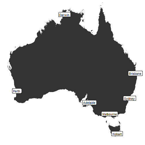
Ok, when you see where Adelaide is you’ll agree that it’s fine to assume Hush and Grandma Poss live in the bush a bit further North from Adelaide. By the way, the only map of the trip I found online does not seem to show their home address. Maybe because they do not want the possum stars to have to deal with too many visitors?
I also notice I only get no occurrence from the Northern hairy-nosed wombat but it seems to be rarer than the common wombat (ok, the name might have been a good clue for me before I got the data).
Geocoding the cities
The cities we need to geocode, and the food eaten by Hush and Grandma Poss while visiting them, are:
cities <- tibble::tibble(city = c("Adelaide", "Melbourne",
                                  "Sydney", "Brisbane",
                                  "Darwin", "Perth",
                                  "Hobart"),
                         food = c("Anzac biscuit", "mornay and Minties",
                                  "steak and salad", "pumpkin scones",
                                  "vegemite", "pavlova",
                                  "lamington"))

knitr::kable(cities)
| city | food |
|---|---|
| Adelaide | Anzac biscuit |
| Melbourne | mornay and Minties |
| Sydney | steak and salad |
| Brisbane | pumpkin scones |
| Darwin | vegemite |
| Perth | pavlova |
| Hobart | lamington |
We shall perfom geocoding using my own package opencage which is a wrapper for R of the OpenCage API. This package was reviewed by Julia Silge for rOpenSci.
library("opencage")
get_lozcation <- function(city){
  opencage_results <- opencage::opencage_forward(placename = city,
                                                 countrycode = "AU")
  output <- opencage_results$results
  output$city <- city
  output <- output[!is.na(output$components.city),]
  output <- output[output$components.city == city,]
  if(nrow(output) > 1){
    output <- output[output$confidence == min(output$confidence),]
  }

  output
}
A small technical note, depending on the font you use in RMarkdown and that sort of encoding joy sources, you now get a flag from the OpenCage API! In my blogging font, it is a bit boring, e.g.:
adelaide <- get_lozcation(city = "Adelaide")
adelaide$annotations.flag gives me 🇦🇺. But still, a cool feature… among other tons of more useful features OpenCage has like the abbr parameter to get shorter names.
Now let’s geocode all cities!
geozcoded_cities <- purrr::map_df(cities$city, get_lozcation)
geozcoded_cities <- dplyr::left_join(geozcoded_cities, cities, by = "city")
Cool, now we can plot them!
ozmap  +
  geom_label(data = geozcoded_cities,
             aes(geometry.lng, geometry.lat,
                 label = city))

Mapping the book!
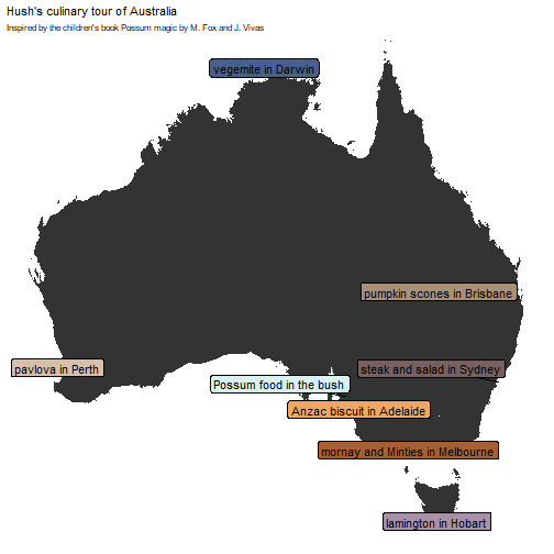
In this last section, I’ll invent a home address for Hush and Grandma Poss and produce an educative map containing both city names and city food specialties! Having 7 cities and one bush location, I’ll use an 8-colour ochRe palette, “namatjira_qual” derived from the beautiful watercolour painting “Twin Ghosts”, by Aboriginal artist Albert Namatjira (again, I’m getting info from this blog post). Here again, no information is conveyed by the color.
library("ggrepel")
hush_home <- tibble::tibble(geometry.lng = adelaide$geometry.lng,
                            geometry.lat = adelaide$geometry.lat + 0.01,
                            city = "the bush",
                            food = "Possum food")

hush_places <- dplyr::bind_rows(geozcoded_cities, hush_home)

ozmap  +
  geom_point(data = hush_places,
              aes(geometry.lng, geometry.lat),
             col = "grey20") +
  geom_label_repel(data = hush_places,
                   aes(geometry.lng + 0.3, geometry.lat + 0.3,
                       label = paste(food, "in", city),
                       fill = city)) +
    scale_fill_ochre(palette = "namatjira_qual") +
  theme(legend.position = "none") +
  ggtitle("Hush's culinary tour of Australia",
          subtitle = "Inspired by the children's book Possum magic by M. Fox and J. Vivas")

Now, I’ll show this map to our baby as soon as he’s old enough to get it, and then we’ll plan a culinary tour of Australia together! Probably not on a bike like Hush and Grandma Poss, unless we can whip up some magic!