2017/10/06

magick / gif / rvest / webscraping / traveling salesperson problem / TSP / mixed integer linear programming / great circles / geosphere / kitsch plot

View source

It was recently brought to my attention by Hannah Frick that there are now sooo many R-Ladies chapters around the world! R-Ladies is a world-wide organization to promote gender diversity in the R community, and I’m very grateful to be part of this community through which I met so many awesome ladies! Since we’re all connected, it has now happened quite a few times that R-Ladies gave talks at chapters outside of their hometowns. An R-Lady from Taiwan giving a talk in Madrid while on a trip in Europe and another one doing the same in Lisbon, an R-Lady from San Francisco presenting at the London and Barcelona chapters thanks to a conference on the continent, an R-Lady from Uruguay sharing her experience for the New York City and San Francisco chapters… It’s like rockstars tours!

Therefore we R-Ladies often joke about doing an exhaustive global tour. Hannah made me think about this tour again… If someone were to really visit all of the chapters, what would be the shortest itinerary? And could we do a cool gif with the results? These are the problems we solve here.

Getting the chapters

To find all chapters, I’ll use Meetup information about meetups whose topics include “r-ladies”, although it means forgetting a few chapters that maybe haven’t updated their topics yet. Thus, I’ll scrape this webpage because I’m too impatient to wait for the cool meetupr package to include the Meetup API topic endpoint and because I’m too lazy to include it myself. I did open an issue though. Besides, I was allowed to scrape the page:

robotstxt::paths_allowed("https://www.meetup.com/topics/")

## [1] TRUE

Yesss. So let’s scrape!

library("rvest")

link <- "https://www.meetup.com/topics/r-ladies/all/"
page_content <- read_html(link)
css <- 'span[class="text--secondary text--small chunk"]'

chapters <-  html_nodes(page_content, css) %>% html_text(trim = TRUE)
chapters <- stringr::str_replace(chapters, ".*\\|", "")
chapters <- trimws(chapters)
head(chapters)

## [1] "London, United Kingdom" "San Francisco, CA"     
## [3] "Istanbul, Turkey"       "Melbourne, Australia"  
## [5] "New York, NY"           "Madrid, Spain"

# Montenegro
chapters[stringr::str_detect(chapters, "Montenegro")] <- "Herceg Novi, Montenegro"

Geolocating the chapters

Here I decided to use a nifty package to the awesome OpenCage API. Ok, this is my own package. But hey it’s really a good geocoding API. And the package was reviewed for rOpenSci by Julia Silge! In the docs of the package you’ll see how to save your API key in order not to have to input it as a function parameter every time.

Given that there are many chapters but not that many (41 to be exact), I could inspect the results and check them.

geolocate_chapter <- function(chapter){
  # query the API
  results <- opencage::opencage_forward(chapter)$results
  # deal with Strasbourg
  if(chapter == "Strasbourg, France"){
    results <- dplyr::filter(results, components.city == "Strasbourg")
  }
  # get a CITY
  results <- dplyr::filter(results, components._type == "city")
  # sort the results by confidence score 
  results <- dplyr::arrange(results, desc(confidence))
  # choose the first line among those with highest confidence score
  results <- results[1,]
  # return only long and lat
  tibble::tibble(long = results$geometry.lng,
                 lat = results$geometry.lat,
                 chapter = chapter, 
                 formatted = results$formatted)
}

chapters_df <- purrr::map_df(chapters, geolocate_chapter)

# add an index variable
chapters_df <- dplyr::mutate(chapters_df, id = 1:nrow(chapters_df))

knitr::kable(chapters_df[1:10,])

long	lat	chapter	formatted	id
-0.1276473	51.50732	London, United Kingdom	London, United Kingdom	1
-122.4192362	37.77928	San Francisco, CA	San Francisco, San Francisco City and County, California, United States of America	2
28.9651646	41.00963	Istanbul, Turkey	Istanbul, Fatih, Turkey	3
144.9631608	-37.81422	Melbourne, Australia	Melbourne VIC 3000, Australia	4
-73.9865811	40.73060	New York, NY	New York City, United States of America	5
-3.7652699	40.32819	Madrid, Spain	Leganés, Community of Madrid, Spain	6
-77.0366455	38.89495	Washington, DC	Washington, District of Columbia, United States of America	7
-83.0007064	39.96226	Columbus, OH	Columbus, Franklin County, Ohio, United States of America	8
-71.0595677	42.36048	Boston, MA	Boston, Suffolk, Massachusetts, United States of America	9
-79.0232050	35.85030	Durham, NC	Durham, NC, United States of America	10

Planning the trip

I wanted to use the ompr package inspired by this fantastic use case, “Boris Johnson’s fully global itinerary of apology” – be careful, the code of this use case is slightly outdated but is up-to-date in the traveling salesperson vignette. The ompr package supports modeling and solving Mixed Integer Linear Programs. I got a not so bad notion of what this means by looking at this collection of use cases. Sadly, the traveling salesperson problem is a complicated problem and its solving time exponentially increases with the number of stops… in that case, it became really too long for plain mixed integer linear programming, as in “more than 24 hours later not done” too long.

Therefore, I decided to use a specific R package for traveling salesperson problems TSP. Dirk, ompr's maintainer, actually used it once as seen in this gist and then in this newspaper piece about how to go to all 78 Berlin museums during the night of the museums. Quite cool!

We first need to compute the distance between chapters. In kilometers and rounded since it’s enough precision.

convert_to_km <- function(x){
  round(x/1000)
}

distance <- geosphere::distm(as.matrix(dplyr::select(chapters_df, long, lat)), fun = geosphere::distGeo) %>% 
  convert_to_km()

I used methods that do not find the optimal tour. This means that probably my solution isn’t the best one, but let’s say it’s ok for this time. Otherwise, the best thing is to ask Concorde’s maintainer if one can use their algorithm which is the best one out there, see its terms of use here.

library("TSP")
set.seed(42)
result0 <- solve_TSP(TSP(distance), method = "nearest_insertion")
result <- solve_TSP(TSP(distance), method = "two_opt",
                    control = list(tour = result0))

And here is how to link the solution to our initial chapters data.frame.

paths <- tibble::tibble(from = chapters_df$chapter[as.integer(result)],
                        to = chapters_df$chapter[c(as.integer(result)[2:41], as.integer(result)[1])], 
                        trip_id = 1:41)
paths <- tidyr::gather(paths, "property", "chapter", 1:2)
paths <- dplyr::left_join(paths, chapters_df, by = "chapter")
knitr::kable(paths[1:3,])

trip_id	property	chapter	long	lat	formatted	id
1	from	Charlottesville, VA	-78.55676	38.08766	Charlottesville, VA, United States of America	38
2	from	Washington, DC	-77.03665	38.89495	Washington, District of Columbia, United States of America	7
3	from	New York, NY	-73.98658	40.73060	New York City, United States of America	5

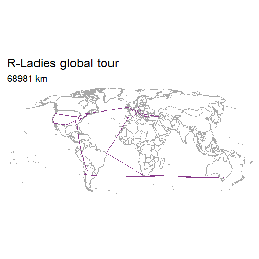
Plotting the tour, boring version

I’ll start by plotting the trips as it is done in the vignette, i.e. in a static way. Note: I used Dirk’s code in the Boris Johnson use case for the map, and had to use a particular branch of ggalt to get coord_proj working.

library("ggplot2")
library("ggalt")
library("ggthemes")
library("ggmap")
world <- map_data("world") %>% dplyr::filter(region != "Antarctica")

ggplot(data = paths, aes(long, lat)) + 
  geom_map(data = world, map = world, aes(long, lat, map_id = region), 
           fill = "white", color = "darkgrey", alpha = 0.8, size = 0.2) + 
  geom_path(aes(group = trip_id), color = "#88398A") + 
  geom_point(data = chapters_df, color = "#88398A", size = 0.8) + 
  theme_map(base_size =20) + 
  coord_proj("+proj=robin +lon_0=0 +x_0=0 +y_0=0 +ellps=WGS84 +datum=WGS84 +units=m +no_defs") + 
  ggtitle("R-Ladies global tour", 
          subtitle = paste0(tour_length(result), " km"))

plot of chunk unnamed-chunk-8

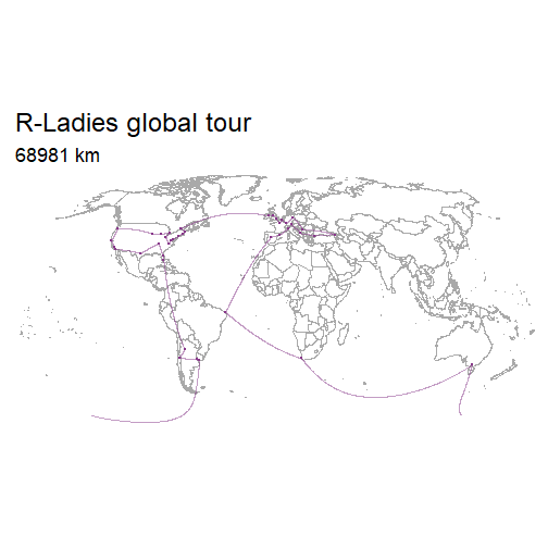
Dirk told me the map would look better with great circles instead of straight lines so I googled a bit around, asked for help on Twitter before finding this post.

library("geosphere")

# find points on great circles between chapters
gc_routes <- gcIntermediate(paths[1:length(chapters), c("long", "lat")],
                            paths[(length(chapters)+1):(2*length(chapters)), c("long", "lat")],
                            n = 360, addStartEnd = TRUE, sp = TRUE, 
                            breakAtDateLine = TRUE)
gc_routes <- SpatialLinesDataFrame(gc_routes, 
                                   data.frame(id = paths$id,
                                              stringsAsFactors = FALSE))
gc_routes_df <- fortify(gc_routes)

p <- ggplot() + 
  geom_map(data = world, map = world, aes(long, lat, map_id = region), 
           fill = "white", color = "darkgrey", alpha = 0.8, size = 0.2) + 
  geom_path(data = gc_routes_df, 
            aes(long, lat, group = group), alpha = 0.5, color = "#88398A") + 
  geom_point(data = chapters_df, color = "#88398A", size = 0.8,
             aes(long, lat)) + 
  theme_map(base_size =20)+ 
  coord_proj("+proj=robin +lon_0=0 +x_0=0 +y_0=0 +ellps=WGS84 +datum=WGS84 +units=m +no_defs")

p + 
  ggtitle("R-Ladies global tour", 
          subtitle = paste0(tour_length(result), " km"))

plot of chunk unnamed-chunk-10

Ok this is nicer, it was worth the search.

Plotting the tour, magical version

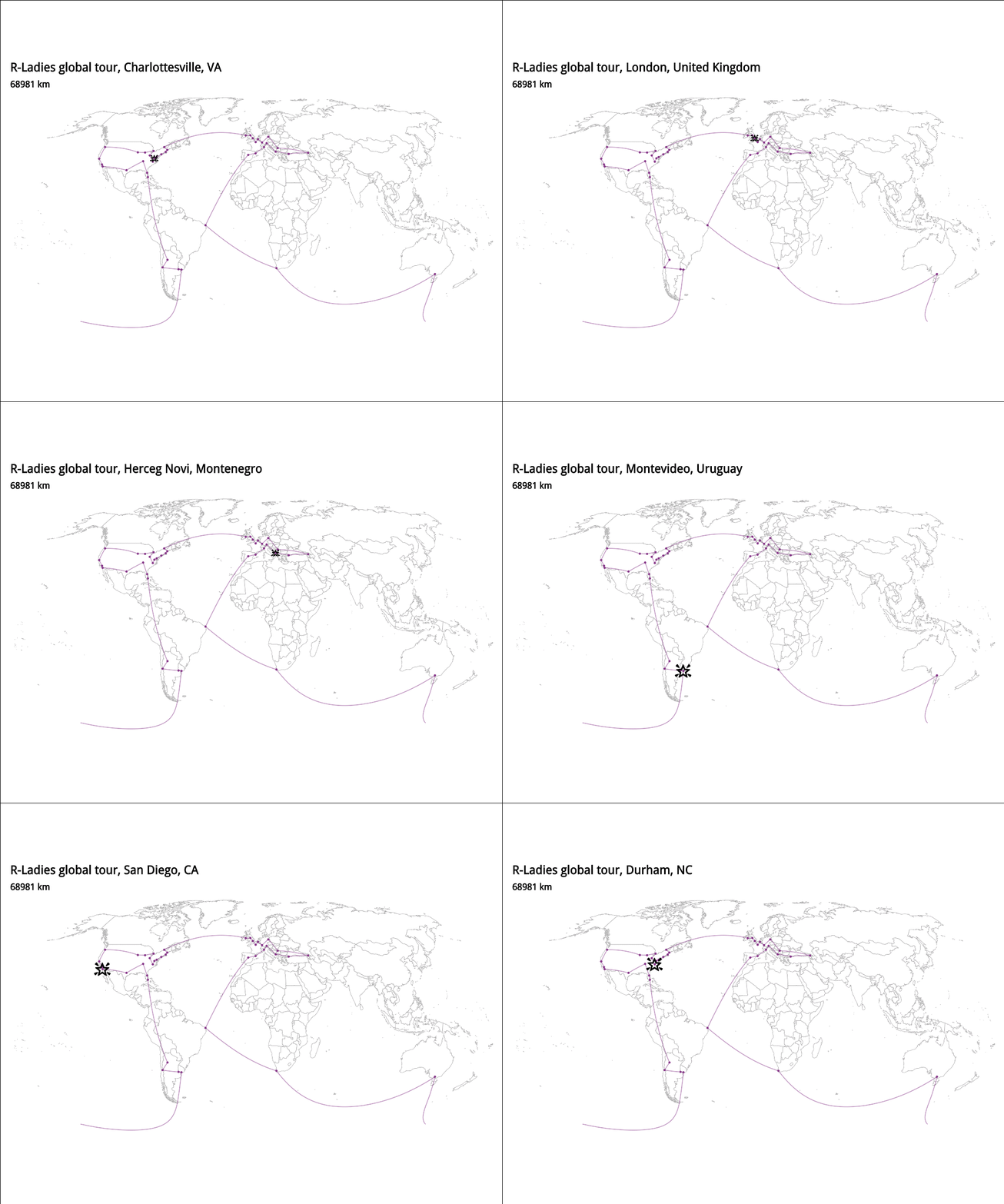
And now I’ll use magick because I want to add a small star flying around the world. By the way if this global tour were to happen I reckon that one would need to donate a lot of money to rainforest charities or the like, because it’d have a huge carbon footprint! Too bad really, I don’t want my gif to promote planet destroying behaviours.

To make the gif I used code similar to the one shared in this post but in a better version thanks to Jeroen who told me to read the vignette again. Not saving PNGs saves time!

I first wanted to really show the emoji flying along the route and even created data for that, with a number of rows between chapters proportional to the distance between them. It’d have looked nice and smooth. But making a gif with hundreds of frames ended up being too long for me at the moment. So I came up with another idea, I’ll have to hope you like it!

library("emojifont")
load.emojifont('OpenSansEmoji.ttf')
library("magick")

plot_one_moment <- function(chapter, size, p,
                            chapters_df){
 
print(p + 
  ggtitle(paste0("R-Ladies global tour, ",
                 chapters_df[chapters_df$chapter == chapter,]$chapter), 
          subtitle = paste0(tour_length(result), " km"))+ 
    geom_text(data = chapters_df[chapters_df$chapter == chapter,], 
            aes(x = long, 
                y = lat,
                label = emoji("star2")),
            family="OpenSansEmoji",
                size = size))


}

img <- image_graph(1000, 800, res = 96)
out <- purrr::walk2(rep(chapters[as.integer(result)], each = 2),
                   rep(c(5, 10), length = length(chapters)*2),
                   p = p,
     plot_one_moment,
      chapters_df = chapters_df) 
dev.off()

## png 
##   2

image_animate(img, fps=1) %>%
  image_write("rladiesglobal.gif")

At least I made a twinkling star. I hope Hannah will be happy with the gif, because now I’d like to just dream of potential future trips! Or learn a bit of geography by looking at the gif.