Last week I published a post about scraping Radio Swiss Classic program. After that, Bob Rudis wrote an extremely useful post improving my code a lot and teaching me cool stuff. I don’t know why I forgot to add pauses between requests… Really bad behaviour! I will use his code today for re-scraping the data.
Why re-scrape the data? I mentioned broken links in my post. In fact, each time I hit a broken page, Radio Swiss Classic webmaster received an email. That person received a lot of emails because of me. They repaired the bug explaining these broken pages and contacted me because someone had turned me in (I feel super famous or spied on now), very kindly mentioning they had fixed all pages, and not holding any grudge against me. So let’s scrape everything again!
Scraping the program
So this is mostly Bob Rudis’ code with my clumsy comments alongside his comments. His are always in-line. I really recommend you to read his post!
library("rvest")
library("purrr")
library("stringi")
library("lubridate")
library("tidyverse")

# using purrr::safely is cool because if the page
# is broken you get NULL as an output
s_read_html <- purrr::safely(read_html)

# helper for brevity
xtract_nodes <- function(node, css) {
  html_nodes(node, css) %>% html_text(trim = TRUE)
}

get_one_day_program <- function(date=Sys.Date(),
                                base_url="http://www.radioswissclassic.ch/en/music-programme/search/%s",
                                pb=NULL) {
  # progress bar magic!
  if (!is.null(pb)) pb$tick()$print()

  # that's the part where you're nice towards the website
  Sys.sleep(sample(seq(0,1,0.25), 1)) # ideally, make this sample(5,1)

  date <- ymd(date) # handles case where input is character ISO date

  pg <- s_read_html(sprintf(base_url, format(date, "%Y%m%d")))

  if (!is.null(pg$result)) {
# go read Bob Rudis' post, in particular to read about
# the extra selector for "playlist"
    dplyr::data_frame(

      date = date,
      time = xtract_nodes(pg$result, 'div[class="playlist"] *
                                            span[class="time hidden-xs"]') %>% hm(),
      datetime = update(date, hour = hour(time), minute = minute(time)),
      artist = xtract_nodes(pg$result, 'div[class="playlist"] * span[class="titletag"]'),
      title = xtract_nodes(pg$result, 'div[class="playlist"] * span[class="artist"]')

    )

  } else {
    closeAllConnections()
    NULL
  }

}

search_dates <- seq(from = ymd("2008-09-01"), to = ymd("2017-04-22"), by = "1 day")

# how you can make the progress bar work,
# estimate the time necessary for 5 requests
pb <- dplyr::progress_estimated(length(search_dates))
programs_df <- map_df(search_dates, get_one_day_program, pb=pb)
programs_df <- programs_df %>%
   dplyr::select(- time) %>%
   dplyr::mutate(datetime = force_tz(datetime, tz = "Europe/Zurich"))
programs_df

save(programs_df, file = "data/radioswissclassic_programs_radioedit.RData")
load("data/radioswissclassic_programs_radioedit.RData")
search_dates <- seq(from = lubridate::ymd("2008-09-01"), to = lubridate::ymd("2017-04-22"), by = "1 day")
This time I got 100% of programs!
Now I can improve my analysis of the data: My colleague Carles (who miiight have been receiving the link to each of my posts because I feel he needs to know about all of them… poor Carles) left a comment on my last post with two nice suggestions.
Applying quantile regression to the duration of pieces
What Carles said: “Regarding differences throughout the day, I agree that there are no major differences on the mean, but there are in the upper quantiles. I’d suggest quantile regression or quantile smoothing in case you want to try ;)”. Let’s not comment on the absence of nose of this smiley, my colleague is a nice guy so I’ll try to not freak out and to concentrate on the statistics.
library("magrittr")
programs_df <- dplyr::arrange(programs_df, datetime)
programs_df <- dplyr::mutate(programs_df,
                          duration = difftime(lead(datetime, 1),
                                       datetime,
                                       units = "min"))

programs_df <- dplyr::mutate(programs_df,
                          duration = ifelse(duration > 60,
                                            NA, duration))
programs_df <- dplyr::mutate(programs_df,
                          hour = as.factor(lubridate::hour(datetime)))

programs_df <- dplyr::mutate(programs_df,
                             night = (lubridate::hour(datetime) <= 4 | lubridate::hour(datetime) >= 20))


quantiles <- function(x){
  probs <- seq(from = 0.5, to = 0.95, by = 0.05)
  quantiles_names <- paste0("q", probs*100)
  quantiles <- purrr::map_dbl(probs, function(p, v = x){
    quantile(v, probs = p, na.rm = TRUE)
  })
  df <- tibble::as.tibble(t(quantiles))
  names(df) <- quantiles_names
  return(df)
}

programs_df %>%
  dplyr::group_by(night) %>%
  dplyr::summarize(duration_q = list(quantiles(duration))) %>%
  tidyr::unnest(duration_q) %>%
  knitr::kable()
| night | q50 | q55 | q60 | q65 | q70 | q75 | q80 | q85 | q90 | q95 |
|---|---|---|---|---|---|---|---|---|---|---|
| FALSE | 7 | 8 | 8 | 9 | 9 | 10 | 10 | 11 | 13 | 16 |
| TRUE | 8 | 8 | 9 | 9 | 10 | 11 | 13 | 16 | 20 | 26 |
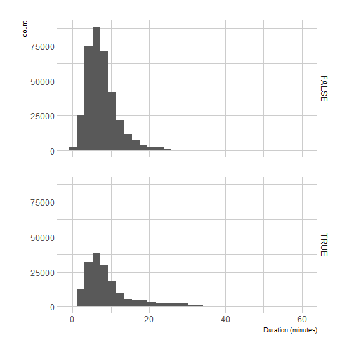
Looking at this table above, it’s true that the upper quantiles of piece duration seem to be longet at night.
library("ggplot2")
library("hrbrthemes")
ggplot(programs_df) +
  geom_histogram(aes(duration)) +
  facet_grid(night ~ .) +
  theme_ipsum() +
  xlab("Duration (minutes)")

And I think these histograms are actually clearer than the boxplots of last post.
So now let’s try quantile regression, which I admit I had never used. The vignette of the quantreg package is really nice, it feels a bit old school with a real introduction and a section called “What is a vignette?”. The vignette starts with this sentence “Beran’s (2003) provocative definition of statistics as ‘the study of algorithms for
data analysis’ elevates computational considerations to the forefront of the field.”. Roger Koenker also writes " Although there is now some functionality for quantile regression in most of the major commercial statistical packages, I have a natural predilection for the R environment and the software that I have developed for R.” which made me smile. Last nice point about the vignette I noticed, it encourages a contributor mindset by saying “When such modifications appear to be of general applicability,
it is desirable to communicate them to the package author, so they could be shared with the larger community.” Ok a real last point about that package, the list of authors includes Brian D Ripley with this note from Roger Koenker “Initial (2001) R port from S (to my everlasting shame – how could I have been so slow to adopt R!”.
In the following I will just look at the effect of night on the duration for various quantiles, nothing fancy.
library("quantreg")

model <- rq(duration ~ night,
            tau = seq(from = 0.5, to = 0.95, by = 0.05),
           data = programs_df,
           method = "pfn")
summaries <- summary(model, se = "ker")

transform_summary <- function(summ){
  coeffs <- tibble::as.tibble(summ$coefficients)
  coeffs <- dplyr::mutate_(coeffs, tau = ~summ$tau)
  coeffs[2,]
}

purrr::map(summaries, transform_summary) %>%
  dplyr::bind_rows() %>%
  knitr::kable()
| Value | Std. Error | t value | Pr(>|t|) | tau |
|---|---|---|---|---|
| 1 | 0.0082075 | 121.83907 | 0 | 0.50 |
| 0 | 0.0082689 | 0.00000 | 1 | 0.55 |
| 1 | 0.0094450 | 105.87571 | 0 | 0.60 |
| 0 | 0.0093682 | 0.00000 | 1 | 0.65 |
| 1 | 0.0106465 | 93.92756 | 0 | 0.70 |
| 1 | 0.0122657 | 81.52811 | 0 | 0.75 |
| 3 | 0.0216791 | 138.38211 | 0 | 0.80 |
| 5 | 0.0298266 | 167.63566 | 0 | 0.85 |
| 7 | 0.0428316 | 163.43057 | 0 | 0.90 |
| 10 | 0.0605325 | 165.20043 | 0 | 0.95 |
This seems to support the idea that upper quantiles of duration are bigger at night. This shift of the distribution of duration at night compared to its distribution during daytime means that there are more long pieces at night… which is what the website claims, so we’re good. Just for info, we are looking at 171668 pieces played at night and 355487 pieces played during the day, that is to say a lot.
Using keywords to identify the speed of pieces
Carles said: “For romantic music the type of composition “Scherzo”/“Waltz”/“Nocturne” may tell you something about the mood of the composition”. Okay, time to analyse some text data then! Instead of looking at the mood of the music as suggested by Carles, I’ll look at the tempo of the pieces instead (from Wikipedia page, see “Italian tempo markings”).
To identify the tempo of each piece indicating one, I shall use fuzzyjoin, a very handy package for joining tables based on say, close geographical coordinates or regular expressions.
tempos <- tolower(c("Larghissimo", "Grave", "Largo",
    "Lento", "Larghetto", "Adagio",
    "Adagietto", "Andante", "Andantino",
    "Marcia moderato", "Andante moderato",
    "Moderato", "Allegretto", "Allegro moderato",
    "Allegro", "Vivace", "Vivacissimo",
    "Allegrissimo", "Presto", "Prestissimo"))
tempos <- tibble::tibble(tempo = tempos,
                         speed = 1:length(tempos))

programs <- dplyr::mutate(programs_df,
                          title = tolower(title))

library("fuzzyjoin")
programs <- regex_inner_join(programs, tempos,
                            by = c(title = "tempo"))
Now I have to take care of pieces that got several tempos, for instance because their title is “grave and allegro blabla” or “something moderato” thus yielding “something” and “something moderato” as tempos. For the first case I’ll randomly sample one of the tempos, for the second case I’ll keep the most precise tempo.
set.seed(1)
nrow(programs)
## [1] 120052
programs <- split(programs, programs$datetime)

clean_tempos <- function(df){
  if(nrow(df) > 1){
    if(any(stringr::str_detect(df$tempo, " moderato"))){
      df <- dplyr::filter_(df, lazyeval::interp(~ stringr::str_detect(df$tempo, " moderato")))
    }else{
      df <- dplyr::sample_n(df, size = 1)
    }

  }
  return(df)

}

programs <- purrr::map(programs, clean_tempos)
programs <- dplyr::bind_rows(programs)
nrow(programs)
## [1] 102439
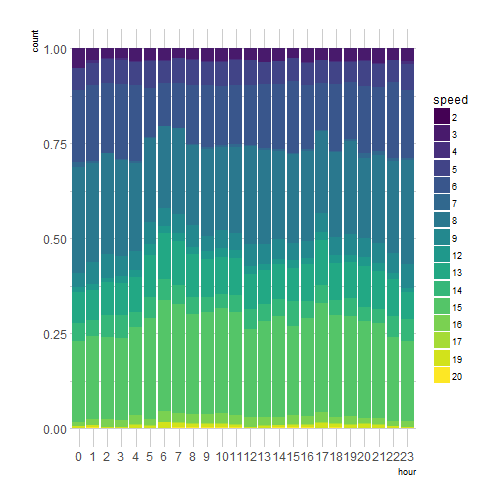
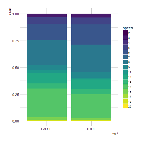
Now that we have 102439 pieces with a known speed out of 527168, let’s look at speed distribution depending on the hour of the day.
programs %>%
  dplyr::group_by(night) %>%
  dplyr::summarize(mean_speed = mean(speed),
            median_speed = median(speed)) %>%
  knitr::kable()
| night | mean_speed | median_speed |
|---|---|---|
| FALSE | 10.453073 | 9 |
| TRUE | 9.888101 | 8 |
programs <- dplyr::mutate(programs, speed = as.factor(speed))

library("viridis")

ggplot(programs) +
  geom_bar(aes(hour, fill = speed),
           position = "fill") +
  scale_fill_viridis(discrete = TRUE) +
  theme_ipsum()

ggplot(programs) +
  geom_bar(aes(night, fill = speed),
           position = "fill") +
  scale_fill_viridis(discrete = TRUE) +
  theme_ipsum()

Honestly, I don’t really see a change of speed at night, or only a really small one, so my method was probably not a very good way of estimating the liveliness of pieces.
Conclusion
I’d like to say thanks again to Bob Rudis, to Radio Swiss Classic webmaster and to my colleague Carles. I was also surprised and happy to receive an email from a university music theory teacher, who told me he could use such data in class to look at popular music pieces. I really like how this blogging thing makes me discover new fields!