As described in my last post, I extracted all notable deaths from Wikipedia over the 2004-2016 period. In this post I want to explore this study population. Who were the notable dead?
How old were notable dead?
Let me assume here most entries of the table are humans. I won’t make the effort to remove dogs or horses from the list yet, which introduces a small mistake.
library("ggplot2")
library("viridis")
library("broom")
library("dplyr")
library("lubridate")
library("tidytext")
library("rcorpora")
deaths <- readr::read_csv("data/deaths_with_demonyms.csv")
As a reminder, in case you didn’t learn the figures from my last post (shame on you), the table contains information about 56303 notable deaths. I could extract the age of 97% of them.
ggplot(deaths) +
  geom_histogram(aes(age)) +
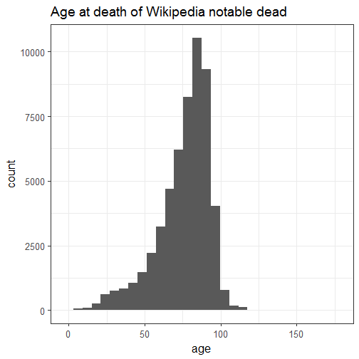
  ggtitle("Age at death of Wikipedia notable dead")

Let’s be honest, I expected a bimodal distribution with a first peak at 27.
tidy(summary(deaths$age))
##   minimum q1 median  mean q3 maximum   na
## 1       1 68     80 75.94 88     176 1677
Wow this is a really high maximal age.
arrange(deaths, desc(age)) %>%
  head(n = 10) %>%
  knitr::kable()
| wiki_link | name | age | country_role | date | country | adj_length | adjectivals | occupation |
|---|---|---|---|---|---|---|---|---|
| Harriet_(tortoise) | Harriet (tortoise) | 176 | NA | 2006-06-23 | NA | NA | NA | NA |
| Eisenhower_Tree | Eisenhower Tree | 125 | American | 2014-02-16 | United States | 1 | American | NA American |
| J%C3%B3zef_Piotrowski_(organist) | Józef Piotrowski (organist) | 118 | Polish organist and longevity claimant. | 2005-09-08 | Poland | 1 | Polish .* | organist and longevity claimant |
| Misao_Okawa | Misao Okawa | 117 | Japanese supercentenarian | 2015-04-01 | Japan | 1 | Japanese .* | supercentenarian |
| Pawe%C5%82_Parniak | Pawel Parniak | 116 | Polish supercentenarian | 2006-03-27 | Poland | 1 | Polish .* | supercentenarian |
| Gertrude_Weaver | Gertrude Weaver | 116 | American | 2015-04-06 | United States | 1 | American | NA American |
| Jai_Gurudev | Jai Gurudev | 116 | Indian religious leader. | 2012-05-18 | India | 1 | Indian .* | religious leader |
| Susannah_Mushatt_Jones | Susannah Mushatt Jones | 116 | American | 2016-05-12 | United States | 1 | American | NA American |
| Jiroemon_Kimura | Jiroemon Kimura | 116 | Japanese | 2013-06-12 | Japan | 1 | Japanese .* | NA Japanese |
| Jeralean_Talley | Jeralean Talley | 116 | American supercentenarian | 2015-06-17 | United States | 1 | American | supercentenarian |
Ok, so the oldest beings in this table were a tortoise and a tree, which we might want to remove from the rest of the analysis.
deaths <- filter(deaths, age < 125)
What about the deaths at the youngest ages?
arrange(deaths, age) %>%
  head(n = 10) %>%
  knitr::kable()
| wiki_link | name | age | country_role | date | country | adj_length | adjectivals | occupation |
|---|---|---|---|---|---|---|---|---|
| Manar_Maged class=mw-redirect | Manar Maged | 1 | Egyptian girl born with two heads | 2006-03-26 | Egypt | 1 | Egyptian .* | girl born with two heads |
| Ayelet_Galena | Ayelet Galena | 2 | American child | 2012-01-31 | United States | 1 | American | child |
| Colonel_Meow | Colonel Meow | 2 | American Himalayan-Persian cat | 2014-01-29 | United States | 1 | American | Himalayan-Persian cat |
| Ben_Bowen | Ben Bowen | 2 | American child cancer victim | 2005-02-25 | United States | 1 | American | child cancer victim |
| Marius_(giraffe) | Marius (giraffe) | 2 | Danish giraffe | 2014-02-09 | Denmark | 1 | Danish .* | giraffe |
| Disappearance_of_Aisling_Symes class=mw-redirect | Disappearance of Aisling Symes | 2 | New Zealand child whose disappearance initiated major search | 2009-10-05 | New Zealand | 2 | New Zealand .* | child whose disappearance initiated major search |
| Paul_the_Octopus | Paul the Octopus | 2 | British-born | 2010-10-26 | NA | NA | NA | British-born |
| Chriselliam | Chriselliam | 3 | Irish-bred British-trained Thoroughbred racehorse | 2014-02-07 | NA | NA | NA | Irish-bred British-trained Thoroughbred racehorse |
| Eight_Belles | Eight Belles | 3 | American racehorse | 2008-05-03 | United States | 1 | American | racehorse |
| Sybil_(cat) | Sybil (cat) | 3 | British Downing Street cat | 2009-07-27 | England | 1 | British .* | Downing Street cat |
As one could have expected, the deaths at youngest ages are some sad stories, about humans but also animals.
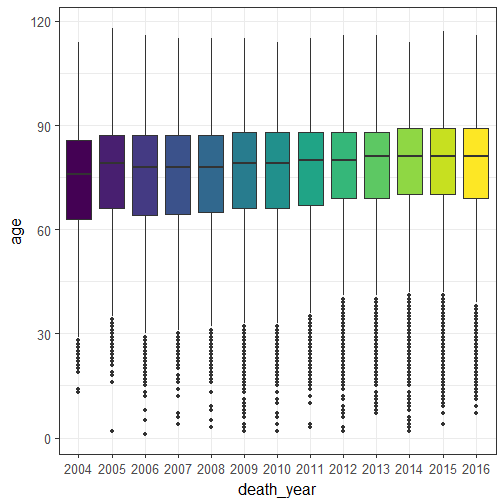
Did the age distribution change over time?
deaths <- mutate(deaths, death_year = as.factor(year(date)))
ggplot(deaths) +
  geom_boxplot(aes(death_year, age, fill = death_year)) +
  scale_fill_viridis(discrete = TRUE) +
  theme(legend.position = "none")

Well maybe there is an increasing trend? I wouldn’t be surprised if it were the case, since life expectancy tends to increase. I first wrote I wouldn’t take the time to test the trend and then I had a very interesting discussion with Miles McBain and Nick Tierney. I had first thought of a linear model, then of a survival analysis but I only have positive events. While using a linear model or a GLM the residuals were never normally distributed. Then Miles mentioned non-parametric tests which is something I never think about. Googling a bit around I fount the Mann-Kendall test!
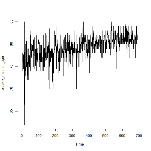
I’m quite lucky I want to see if age at death monotically increases over time because that seems to be the usual use case for it. I choose to use the time series of weekly median age, which I’m not too sure is the best choice. I could have chosen monthly average age, etc.
library("trend")
library("lubridate")
weekly_median_age <- deaths %>%
  filter(!is.na(age)) %>%
  group_by(wiki_link) %>%
  mutate(week = paste(year(date), week(date))) %>%
  group_by(week) %>%
  summarize(age = median(age)) %>% .$age
weekly_median_age <- as.ts(weekly_median_age)
plot(weekly_median_age)

res <- mk.test(weekly_median_age)
summary.trend.test(res)
## Mann-Kendall Test
##
## two-sided homogeinity test
## H0: S = 0 (no trend)
## HA: S != 0 (monotonic trend)
##
## Statistics for total series
##       S     varS    Z   tau     pvalue
## 1 79925 36111378 13.3 0.337 < 2.22e-16
Using this test I have now more support for the existence of a trend, but not for its direction. The same package has an implementation of Sen’s method to compute the slope.
sens <- sens.slope(weekly_median_age, level = 0.95)
sens
##
## Sen's slope and intercept
##
##
## slope:  0.0065
## 95 percent confidence intervall for slope
## 0.0074 0.0056
##
## intercept: 77.1831
## nr. of observations: 689
With such a slope in one year one gains 0.34 years. Will we soon have humans as old as Harriet the tortoise?
Where did notable dead come from?
deaths %>% group_by(country) %>%
  summarize(n = n()) %>%
  arrange(desc(n)) %>%
  head(n = 10) %>%
  knitr::kable()
| country | n |
|---|---|
| United States | 20220 |
| England | 6163 |
| Canada | 2183 |
| Australia | 1783 |
| India | 1604 |
| France | 1277 |
| Germany | 1277 |
| Italy | 1141 |
| Russia[15] | 884 |
| NA | 857 |
Unsurprisingly given what I imagine to be the countries of Wikipedia contributors in English, mostly from developped countries, and then India is a huge English-speaking country. It’d probably be interesting to repeat the same data extraction for all languages and see how we rather know celebrities speaking our own language or sharing our culture.
What were the reasons of notability?
I first played with the idea of using my monkeylearn package to associated an industry to each occupation/reason for being notable, but I soon realized the description was too short for the extractor. I also soon saw I wouldn’t be able to find a good list of jobs, so I resorted to simply look for the most present terms using tidytext. For removing the stop-words I used rcorpora.
stopwords <- corpora("words/stopwords/en")$stopWords

deaths_words <- deaths %>%
  unnest_tokens(word, occupation) %>%
  count(word, sort = TRUE) %>%
  filter(!word %in% stopwords)


head(deaths_words, n = 10) %>%
  knitr::kable()
| word | n |
|---|---|
| politician | 6285 |
| player | 4251 |
| actor | 2807 |
| footballer | 2022 |
| football | 1899 |
| actress | 1693 |
| singer | 1593 |
| writer | 1526 |
| american | 1476 |
| olympic | 1396 |
From these 10 most prevalent terms we could assume being a politician, some sort of athlete (player could also be a football player) or artist can make you notable. It’s interesting to see there are far more actors than actresses. In case you didn’t get the message, in the table there are 756 businessmen, 44 businesswomen, 4 business persons.
I also noticed that there are 147 murderers and 41 serial killers vs. 232 chemists and 46 statisticians. Since the term “data scientist” is quite young, there is none in my table, and I sure wish you’ll all stay healthy, my friends! In the next post I’ll present the analysis of the time series of monthly count of deaths.
If you liked learning more about notable dead, you can have a look at the analysis Hazel Kavili started doing of celebrity deaths in 2016.
I’d like to end this post with a note from my husband, who thinks having a blog makes me an influencer. If you too like Wikipedia, consider donating to the Wikimedia foundation.