I was lucky enough to get some nice and interesting feedback on my last post. One comment was really useful and pretty embarrassing: I had written “see” instead of “sea” in the whole post… Thanks Steve Dempsey for the correction! I also got some questions which I decided to explore.
More water?
I had chosen to look specifically for a few rivers but one commenter, actually Steve Dempsey again, asked me how it would look like if I systematically retrieved all placenames with “sur-”, “upon”, because where he lived in France there were many “sur-Dronne” or “sur l’Isle”. He actually asked the question in French, “Je me demande ce que ça donne avec tous les places avec un “-sur”. Là, où j’étais en France il y avait plein de “-sur-Dronne” ou “-sur-l’Isle”." Let’s see! (or sea? just kidding)
library("dplyr")
library("tidyr")
library("readr")
library("purrr")
ville <- read_tsv("data/2017-01-24-kervillebourg_FR.txt", col_names = FALSE)[, c(2, 5, 6)]
names(ville) <- c("placename", "latitude", "longitude")
ville <- unique(ville)
upon <- filter(ville, grepl("sur-", placename))
If truth be told, I thought I’d just need to filter the relevant placenames and then get nice rivers on my map… nope. So I soon realized I should first find unique names of rivers, then group them by name and only draw the ones that have enough places for the map to be at least a bit pretty.
upon <- by_row(upon, function(df){
  sub(".*sur-", "", df$placename)
}, .to = "waterthing", .collate = "cols")
knitr::kable(head(upon))
| placename | latitude | longitude | waterthing |
|---|---|---|---|
| Domecy-sur-le-Vault | 47.49084 | 3.80953 | le-Vault |
| Yzeures-sur-Creuse | 46.78609 | 0.87166 | Creuse |
| Yville-sur-Seine | 49.39938 | 0.87750 | Seine |
| Wingen-sur-Moder | 48.91900 | 7.37955 | Moder |
| Willer-sur-Thur | 47.84392 | 7.07223 | Thur |
| Wavrans-sur-Ternoise | 50.41322 | 2.30002 | Ternoise |
Let’s see what the more frequent watherthings are:
group_by(upon, waterthing) %>%
  summarize(n = n()) %>%
  arrange(desc(n)) %>%
  head(n = 20) %>%
  knitr::kable()
| waterthing | n |
|---|---|
| Mer | 214 |
| Loire | 152 |
| Seine | 148 |
| Marne | 117 |
| Meuse | 88 |
| Saône | 70 |
| Sarthe | 50 |
| Aube | 44 |
| Cher | 41 |
| Orne | 39 |
| Seille | 39 |
| Moselle | 36 |
| Eure | 34 |
| Yonne | 33 |
| Oise | 32 |
| Vienne | 31 |
| Garonne | 30 |
| Dordogne | 28 |
| Aisne | 26 |
| Allier | 24 |
So I find “Sea” again, and the rivers I had chosen in the last post, and others, whose names I all knew so they must be quite important. I want to keep only the rivers with “enough”” places to make the map pretty, because at the scale of the country I prefer seeing a longer river.
upon <- group_by(upon, waterthing)
upon <- filter(upon, n() >= 25)
upon <- ungroup(upon)
library("ggplot2")
library("ggmap")
library("viridis")
library("ggthemes")
map <- ggmap::get_map(location = "France", zoom = 6, maptype = "watercolor")
This time the map will be really artsier than useful since I’ll have a color by river but no legend because of the higher numbers of rivers.
p <- ggmap(map) +
  geom_point(data = upon,
             aes(x = longitude, y = latitude,
                 col = waterthing), size = 1.3) +
  theme_map()+
  scale_colour_grey(end = 0.7)+
  ggtitle("French placenames containing the word 'sur'") +
  theme(plot.title = element_text(lineheight=1, face="bold"))+
  theme(text = element_text(size=14),
        legend.position = "none")
p
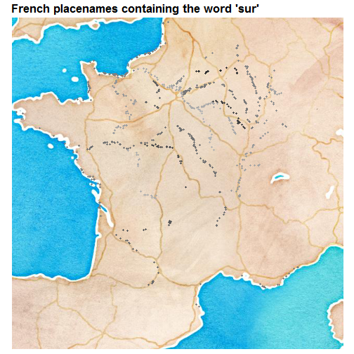
I like this map because I could find the rivers again without having to enter their names, and it looks like drawing with a pencil on watercolor without making any effort. However, since I’m not very good in geography, I’d like to add labels to each river, let’s say somewhere in the middle of the river. I’ll use ggrepel to avoid having overlapping labels. My definition of “somewhere in the middle” is sorting the places of a river by latitude and longitude and then choosing a place close to the middle.
library("ggrepel")
named_upon <- arrange(upon, latitude, longitude)
named_upon <- group_by(named_upon, waterthing)
named_upon <- mutate(named_upon, index = 1:n())
named_upon <- mutate(named_upon, name = ifelse(index == floor(n()/2),
                                   waterthing, NA))
p + geom_label_repel(aes(x = longitude,
                   y = latitude,
                   label = name,
                   max.iter = 20000),
               data = named_upon)
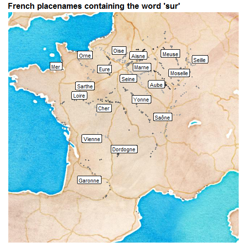
Okay, I’ll now look at the map and learn the names! I’ve lived near the Loire, near the Seine and near the Marne. It might be surprising not to see the Rhine on that map, but placenames in Alsace are often more Germanic, so that would be another story.
Which saints?
I also got questions about saints, one on Twitter from Andrew Boa and a few ones from Andrew MacDonald.
Andrew Boa’s question was the easiest one: how many unique names of saints are there? The questions of the other Andrew were “I wonder, would it be possible to also obtain data on how old these towns are? It would be interesting to see if the gender of popular saints changes over time. Or, more simply, which saints have the most towns? I imagine there are tons of “Saint Sernin"s in the South, and probably lots of “Jeanne-d’Arc"s all over”. Let me tell you I am thankful for the more simply part of the questions because I have no idea where one would find information about the age of the places. Nonetheless, this would be really interesting.
Let’s answer the questions about the number of unique names and their frequencies. I am now in particular curious about André since I got questions from two Andrew’s.
Note that for finding the name I remove the “Saint-” or “Sainte-” part but also everything that could come after another hyphen and a space, e.g. in “Alban-de-Varèze” which I want as “Alban”. Also note that in this analysis I ignore homonym saints, and that Jeanne d’Arc might be a saint, the places named after her don’t contain the word “sainte”.
saints <- ville %>%
  mutate(saint = grepl("Saint-", placename))  %>%
  mutate(sainte = grepl("Sainte-", placename))  %>%
  gather("gender", "yes", saint:sainte) %>%
  filter(yes == TRUE) %>%
  select(- yes)
saints <- by_row(saints, function(df){
  if(df$gender == "saint"){
    name <- sub(".*Saint-", "", df$placename)
  }else{
    name <- sub(".*Sainte-", "", df$placename)
  }
  name <- trimws(name)
  name <- strsplit(name, "-")[[1]][1]
  name <- strsplit(name, " ")[[1]][1]
  return(name)
}, .to = "saintname", .collate = "cols")
knitr::kable(head(saints))
| placename | latitude | longitude | gender | saintname |
|---|---|---|---|---|
| Ygos-Saint-Saturnin | 43.97651 | -0.73780 | saint | Saturnin |
| Canal de Vitry-le-François à Saint-Dizier | 48.73333 | 4.60000 | saint | Dizier |
| Vitrac-Saint-Vincent | 45.79585 | 0.49356 | saint | Vincent |
| Vineuil-Saint-Firmin | 49.20024 | 2.49567 | saint | Firmin |
| Villotte-Saint-Seine | 47.42893 | 4.70571 | saint | Seine |
| Villiers-Saint-Denis | 49.00000 | 3.26667 | saint | Denis |
How many unique names do we have?
group_by(saints, gender) %>%
  summarize(n_names = length(unique(saintname)),
            n_places = n()) %>%
  knitr::kable()
| gender | n_names | n_places |
|---|---|---|
| saint | 1205 | 10310 |
| sainte | 157 | 971 |
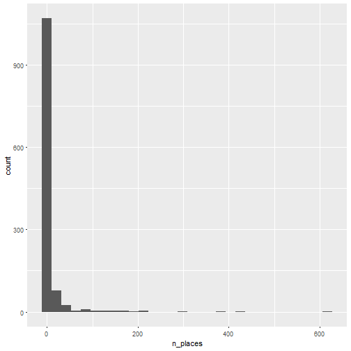
Let’s look at the distributions of number of places by saint name, separately for saints then saintes.
saints_freq <- group_by(saints, gender, saintname)
saints_freq <- summarize(saints_freq, n_places = n())

filter(saints_freq, gender == "saint") %>%
ggplot() +
  geom_histogram(aes(n_places))
## `stat_bin()` using `bins = 30`. Pick better value with `binwidth`.
filter(saints_freq, gender == "sainte") %>%
ggplot() +
  geom_histogram(aes(n_places))
## `stat_bin()` using `bins = 30`. Pick better value with `binwidth`.
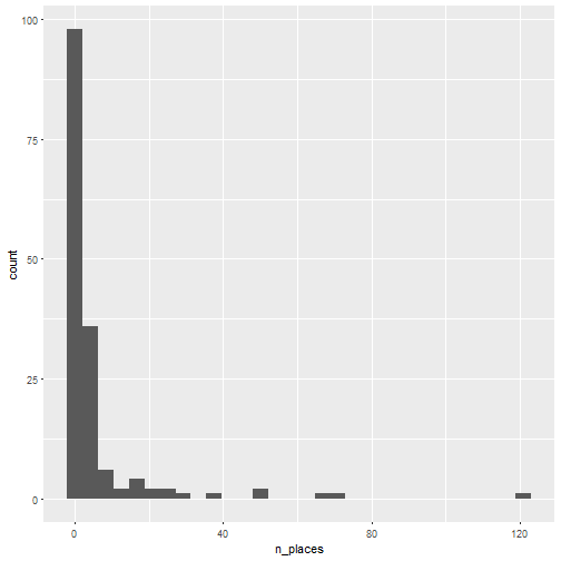
The information I get from looking at these ugly histograms is that there are some names that are very popular and a lot of them that are rarely used. Let’s look at the 11 more popular ones for saints and saintes. Don’t ask me why I chose 11!
arrange(saints_freq, desc(n_places)) %>%
  filter(gender == "saint") %>%
  head(n = 11) %>%
  knitr::kable()
| gender | saintname | n_places |
|---|---|---|
| saint | Martin | 618 |
| saint | Jean | 416 |
| saint | Pierre | 391 |
| saint | Germain | 304 |
| saint | Julien | 219 |
| saint | Laurent | 215 |
| saint | Georges | 214 |
| saint | Hilaire | 181 |
| saint | Aubin | 169 |
| saint | Michel | 168 |
| saint | André | 164 |
So for saints I see names that are still common in France. And André as 11th one, which might explain why I chose the 11 most popular ones…
arrange(saints_freq, desc(n_places)) %>%
  filter(gender == "sainte") %>%
  head(n = 11) %>%
  knitr::kable()
| gender | saintname | n_places |
|---|---|---|
| sainte | Marie | 122 |
| sainte | Croix | 69 |
| sainte | Colombe | 68 |
| sainte | Marguerite | 52 |
| sainte | Anne | 50 |
| sainte | Foy | 36 |
| sainte | Eulalie | 29 |
| sainte | Gemme | 25 |
| sainte | Geneviève | 24 |
| sainte | Catherine | 21 |
| sainte | Radegonde | 20 |
I’m fascinated by some names like Radegonde that are not common any longer.
And since looking at rare names is so fun (isn’t it?), let’s look at the 11th of the least popular names.
arrange(saints_freq, n_places) %>%
  filter(gender == "saint") %>%
  head(n = 11) %>%
  knitr::kable()
| gender | saintname | n_places |
|---|---|---|
| saint | Aaron | 1 |
| saint | Alexis | 1 |
| saint | Alvard | 1 |
| saint | Amas | 1 |
| saint | Amond | 1 |
| saint | Anastase | 1 |
| saint | Andre´ | 1 |
| saint | Andrieu | 1 |
| saint | Andrieux | 1 |
| saint | Anne | 1 |
| saint | Apoll | 1 |
I think some rare names might be errors of accents, e.g. Andre might be André and seeing Anne in the list of saints I’m now wondering about the number of female names classified as saints in the dataset. There are 10 “Saint Mary” in the dataset and 122 “Sainte Marie” so I think the gender inbalance would still exist when accounting for this, but it’s certainly a good point to keep in mind when using this Geonames dataset! If I were to really tackle the issue, I think I’d try using the genderizer package on names, although I’m not so sure it’d perform well for French old names and the rOpensci gender package doesn’t have an historical dataset for France (yet?). I could also simply look for a very French dataset of place names, and hope no name would be translated in it.
Beside discovering this limitation of the dataset, I liked the names one can see by browsing the least popular saint names, like Eusoge or Exupère.
arrange(saints_freq, n_places) %>%
  filter(gender == "sainte") %>%
  head(n = 11) %>%
  knitr::kable()
| gender | saintname | n_places |
|---|---|---|
| sainte | Ame | 1 |
| sainte | Assise | 1 |
| sainte | Avoye | 1 |
| sainte | Awawa | 1 |
| sainte | Blaizine | 1 |
| sainte | Clotilde | 1 |
| sainte | Élisabeth | 1 |
| sainte | Éturien | 1 |
| sainte | Eugienne | 1 |
| sainte | Eulard | 1 |
| sainte | Genevieve | 1 |
This is similarly fascinating and also shows me it might be interesting to re-analyse the all dataset without diacritical accents (Genevieve should be Geneviève).
And Saint Maël, you might ask? Well Maël or Maëlle are Breton names so there’s no place called Saint Maël in the dataset like my holy patron, but there is Maël-Carhaix and Maël-Pestivien. I can’t speak Breton, Wikipedia tells me that Pestivien means “the end of the sources” and for Carhaix it seems to be a long story. After looking at this dataset, I have the impression that the more toponomy questions one tries to answer, the more new questions one has. While this is awesome because of all the learning it implies, I’ll conclude this post (and probably my hobby career as a toponomist :)) by simply plotting the Jeanne d’Arc places for Andrew MacDonald, and Domrémy-la-Pucelle where she was born. There was no Saint-Sermin!
ville <- mutate(ville, jeanne = grepl("Jeanne [dD].[aA]rc", placename))
ville <- mutate(ville, domremy = (placename == "Domrémy-la-Pucelle"))
jeanne <- filter(ville, jeanne | domremy)
jeanne <- tidyr::gather(jeanne, "word", "value", jeanne:domremy)
jeanne <- filter(jeanne, value)
ggmap(map) +
  geom_point(data = jeanne,
             aes(x = longitude, y = latitude, col = word), size = 3) +
  theme_map()+
  ggtitle("French placenames containing 'Jeanne d'Arc'") +
  theme(plot.title = element_text(lineheight=1, face="bold")) +
  scale_color_viridis(discrete = TRUE)
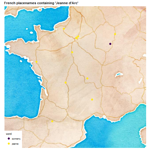
So there are a few Jeanne d’Arc places all over as predicted by Andrew, none very close to Domrémy-la-Pucelle but then this was called Domrémy the virgin after her already.
If you want to play with the dataset yourself, you’ll find it on Geonames, see this gist and in the data folder of this Github repo. If you do, don’t hesitate to share your findings!