Sort of introduction to this post and hopefully the next ones
I usually don’t have any New Year resolution. However, recent tweets about productivity – from people I actually find productive and inspiring – made me ponder a bit on my unfinished side projects. My main 2016 side-project was submitting and defending my PhD thesis, and I’ve written a few R packages, so I’m overall quite happy.
But in 2016 I also started stuff without delivering. In particular, I prepared small data projects in Github repositories with a very precise README because I didn’t have a blog and planned to start one after my PhD thesis. Then I created my blog (thanks Nick!) and… only re-posted an analysis of mine from another blog. My nice repositories are still lying around and they represent quite a few of my West Side-project Story unfinished buildings. I’ve decided transforming some of my usable data projects into blog posts was a nice step towards being or at least feeling more productive.
Let’s start today with my visualizations of names of French places!
Note: the analysis was originally prepared here and advertised on Twitter
Inspired by this work about names of places in Germany, I wanted to have a look at the names of French places. I decided against looking at prefixes and suffixes because I got a more poetical idea: looking for water and saints in my home country.
I got a file of all French places names and geolocation from Geonames. Thanks to Bob Rudis for providing me with the link. The data is distributed under this license.
A first look at the data
library("dplyr")
library("tidyr")
library("readr")
ville <- read_tsv("data/2017-01-24-kervillebourg_FR.txt", col_names = FALSE)[, c(2, 5, 6)]
names(ville) <- c("placename", "latitude", "longitude")
knitr::kable(head(ville))
| placename | latitude | longitude |
|---|---|---|
| Recon, Col de | 46.30352 | 6.82838 |
| Lucelle | 47.41667 | 7.50000 |
| Les Cornettes de Bise | 46.33333 | 6.78333 |
| Ruisseau le Lertzbach | 47.58333 | 7.58333 |
| Le Cheval Blanc | 46.05132 | 6.87178 |
| Jougnena | 46.71667 | 6.40000 |
Names of rivers and sea
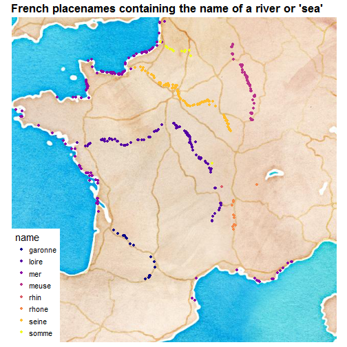
Here I selected names of towns and places that include the names of a few rivers in France, or the word “sea” (“sur-Mer”). This is by no mean an exhaustive representation of such names since I only chose a few rivers and a single pattern of name.
I created new variables that are Booleans by looking for given pattern in names, like “sur-Mer”, then I only filtered the lines where one of the pattern was found, and used tidyr::gather function to end up with the long format you see below.
water <- ville %>%
  mutate(mer = grepl("sur-Mer", placename))  %>%
  mutate(rhone = grepl("sur-Rhône", placename))  %>%
  mutate(somme = grepl("sur-Somme", placename))  %>%
  mutate(loire = grepl("sur-Loire", placename)) %>%
  mutate(seine = grepl("sur-Seine", placename)) %>%
  mutate(rhin = grepl("sur-Rhin", placename)) %>%
  mutate(garonne = grepl("sur-Garonne", placename)) %>%
  mutate(meuse = grepl("sur-Meuse", placename)) %>%
  gather("name", "yes", mer:meuse) %>%
  filter(yes == TRUE) %>%
  select(- yes)
knitr::kable(head(water))
| placename | latitude | longitude | name |
|---|---|---|---|
| Villers-sur-Mer | 49.32264 | 0.00027 | mer |
| Villefranche-sur-Mer | 43.70470 | 7.30776 | mer |
| Vierville-sur-Mer | 49.37237 | -0.90709 | mer |
| Veulettes-sur-Mer | 49.85162 | 0.59719 | mer |
| Ver-sur-Mer | 49.32987 | -0.53118 | mer |
| Vaux-sur-Mer | 45.64606 | -1.05841 | mer |
Then I made an artsy map thanks to the "watercolor" maptype of ggmap and to my beloved viridis. The zoom I chose makes the map only for the métrople, I don’t even include Corsica.
library("ggplot2")
library("ggmap")
library("viridis")
library("ggthemes")
map <- ggmap::get_map(location = "France", zoom = 6, maptype = "watercolor")
ggmap(map) +
  geom_point(data = water,
             aes(x = longitude, y = latitude, col = name)) +
  scale_color_viridis(discrete = TRUE, option = "plasma")+
  theme_map()+
  ggtitle("French placenames containing the name of a river or 'sea'") +
  theme(plot.title = element_text(lineheight=1, face="bold"))+
  theme(text = element_text(size=14))

It was also, I must say, a nice lesson in French geography for me.
Saint et Saintes
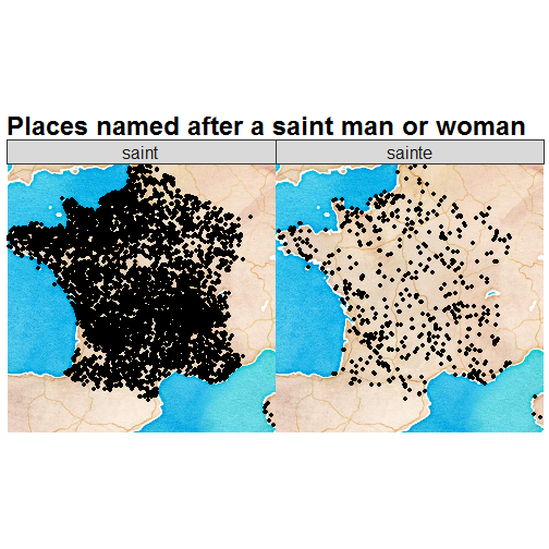
In French, towns such as “Saint-Ouen” and “Sainte-Anne” can easily be partitioned into cities named after a saint man (saint) and cities named after a saint woman (sainte). Thinking of this prompted me to have a look at the distribution of such place names with a similar strategy than for rivers.
saints <- ville %>%
  mutate(saint = grepl("Saint-", placename))  %>%
  mutate(sainte = grepl("Sainte-", placename))  %>%
  gather("name", "yes", saint:sainte) %>%
  filter(yes == TRUE) %>%
  select(- yes)
knitr::kable(head(saints))
| placename | latitude | longitude | name |
|---|---|---|---|
| Ygos-Saint-Saturnin | 43.97651 | -0.73780 | saint |
| Canal de Vitry-le-François à Saint-Dizier | 48.73333 | 4.60000 | saint |
| Vitrac-Saint-Vincent | 45.79585 | 0.49356 | saint |
| Vineuil-Saint-Firmin | 49.20024 | 2.49567 | saint |
| Villotte-Saint-Seine | 47.42893 | 4.70571 | saint |
| Villiers-Saint-Denis | 49.00000 | 3.26667 | saint |
Here is the result on a map.
ggmap(map) +
  geom_point(data = saints,
             aes(x = longitude, y = latitude)) +
  theme_map()+
  ggtitle("Places named after a saint man or woman") +
  theme(plot.title = element_text(lineheight=1, face="bold")) +
  facet_grid(. ~ name) +
  theme(text = element_text(size=20))

Well, I cannot say I’m surprised!
Back when I published this small work only on Github and Twitter, I was pleasantly surprised to see a more elaborate analysis inspired by mine, so if this post made you curious about analysis of French placenames with R, head to Cérès Carton’s repository! And after this, I’ll just warn you to brace yourself for more old repos recycling from me.