This week, a very promising new R blog was launched, namely the blog of Eric Persson a.k.a as expersso on Twitter. I had really been looking forward to this because expersso’s code screenshots have always been quite cool, so seeing his no longer being limited to them is awesome! His first articles series is about a game, you should really check it out. (PSA: if you post screenshots of R code on Twitter, have a look at Sean Kross’ codefinch package!).
Because I’m a nosy person I asked Eric whether he was Swedish, his last name being quite Swedish-looking in my opinion. He is, which made me wonder about Swedish blog topics and actually decided to use one Swedish topic I came up with, the summer guests of the Swedish radio P1! Every summer since 1959, P1 selects a bunch of famous or interesting people and have them record a bit more than one hour program where they’re free to discuss what they want (important events of their life for instance) and to choose the musical breaks (which you don’t get to listen entirely to in the online version because of copyright stuff). The program is then broadcasted in the summer, one guest a day from the end of June to the beginning of August. There’s even a winter version now but I’ll ignore it because it’s too hot here in Barcelona to even think about winter.
It’s a very cool radio program in my opinion. I discovered it at the end of my 5-month research stay in Gothenburg in 2010 and decided it’d be one way to keep my Swedish skills up to date (my other methods include listening to ABBA in Swedish and reading Camilla Läckberg’s novels). I haven’t listened to that many guests but I really enjoy it when I do, and I like how diverse the list of guests is. In this post, I’ll actually try to have a look at the occupations of the guests via Wikidata!
How to get the data?
In order to answer my question I needed a list of all summer guests, and their occupations. I first thought I’d resort to webscraping P1 website, which would have been a good way to provide expersso with an opportunity to give me some constructive feedback. However after websurfing a bit to assess my options, I realized I could use Wikipedia data obtained through APIs rather than webscraping as in my posts about famous dead people. Here was my strategy.
Getting the list of all summer guests from 1959
I downloaded the table of all summer guests from 1959 from this page, which gave me their names and the dates of their episode(s) – yeah some people are invited back.
# all summer guests
sommargaester <- readr::read_csv("data/p1sommar.csv", col_names = FALSE,
                                 locale = readr::locale(encoding = "latin1"))
knitr::kable(sommargaester[1:10,])
| X1 | X2 | X3 | X4 | X5 | X6 | X7 |
|---|---|---|---|---|---|---|
| Aaro,Lars-Eric | 110714 | NA | NA | NA | NA | NA |
| Abdelhadi,Magdi | 070809 | 120716 | NA | NA | NA | NA |
| Abdulle,Sherihan ‘Cherrie’ | 170706 | NA | NA | NA | NA | NA |
| Abele,Anton | 130725 | NA | NA | NA | NA | NA |
| Abenius,Folke | 800627 | NA | NA | NA | NA | NA |
| Abrahamson,Kjell-Albin | 880809 | NA | NA | NA | NA | NA |
| Ackebo,Lena | 970708 | NA | NA | NA | NA | NA |
| Adami,Zanyar | 060707 | NA | NA | NA | NA | NA |
| Adamo,Amelia | 860806 | 870718 | 080701 | NA | NA | NA |
| Adams,Maud | 920703 | 070805 | NA | NA | NA | NA |
# get their names
sommargaester_names <- unique(sommargaester$X1)

# for putting names in the right order for later queries
transform_name <- function(name){
  paste(stringr::str_split(name, ",",
                           simplify = TRUE)[2],
        stringr::str_split(name, ",",
                           simplify = TRUE)[1])
}

pretty_sommargaester_names <- purrr::map_chr(sommargaester_names, transform_name)
sommargaester_names <- tibble::tibble(name = pretty_sommargaester_names,
                                      X1 = sommargaester_names)
sommargaester <- dplyr::left_join(sommargaester, sommargaester_names,
                                  by = "X1")

sommargaester <- dplyr::select(sommargaester, - X1)
# transform the date
sommargaester <- tidyr::gather(sommargaester, "rep", "date", X2:X7)
sommargaester <- dplyr::group_by(sommargaester, name)
sommargaester <- dplyr::mutate(sommargaester, rep = 1:n())
sommargaester <- dplyr::ungroup(sommargaester)

sommargaester <- dplyr::filter(sommargaester, !is.na(date))
# remove winter
sommargaester <- dplyr::filter(sommargaester, !stringr::str_detect(date, "V"))
# remove repeat episodes
sommargaester <- dplyr::filter(sommargaester, !stringr::str_detect(date, "R"))


# transform the date to a format with a non ambiguous year
sommargaester <- dplyr::mutate(sommargaester, date = as.numeric(date))
sommargaester <- dplyr::mutate(sommargaester, date = ifelse(date > 180000, paste0("19", date),
                                                            ifelse(date < 100000,
                                                                   paste0("200", date),
                                                                   paste0("20", date))))
sommargaester <- dplyr::mutate(sommargaester, pretty_date = lubridate::ymd(date))

knitr::kable(sommargaester[1:10,])
| name | rep | date | pretty_date |
|---|---|---|---|
| Lars-Eric Aaro | 1 | 20110714 | 2011-07-14 |
| Magdi Abdelhadi | 1 | 20070809 | 2007-08-09 |
| Sherihan ‘Cherrie’ Abdulle | 1 | 20170706 | 2017-07-06 |
| Anton Abele | 1 | 20130725 | 2013-07-25 |
| Folke Abenius | 1 | 19800627 | 1980-06-27 |
| Kjell-Albin Abrahamson | 1 | 19880809 | 1988-08-09 |
| Lena Ackebo | 1 | 19970708 | 1997-07-08 |
| Zanyar Adami | 1 | 20060707 | 2006-07-07 |
| Amelia Adamo | 1 | 19860806 | 1986-08-06 |
| Maud Adams | 1 | 19920703 | 1992-07-03 |
Getting Wikidata about the summer guests
Then I read the list of Wikipedia R packages put together by Mikhail Popov, data scientist at the Wikimedia foundation with whom I exchanged a few messages after my Wikipedia deaths posts. These packages were either created by him or by Oliver Keyes and really give you access to plenty of structured data so I was happy to at last give the list a try!
I used WikidataQueryServiceR to access Wikidata via the query language SPARQL. Luckily I didn’t need to actually learn SPARQL, I used the first example of the documentation, getting Douglas Adams’ data and played with this online query tool to see how I could modify it to 1) obtain data in Swedish because Swedish Wikipedia is probably more complete about Swedish people and 2) obtain data about the summer guests, not Douglas Adams. For that second point I needed the item ID of each summer guests which I queried via another R package, WikidataR. I could have modified the SPARQL even more since I wouldn’t be using picture information but I wasn’t in a very perfectionist mood.
Doing all of this I only scraped the surface of the possibilities offered by the Wikipedia-related R packages and can already tell one could do a bunch of exciting analyses with them!
Note that I used Bob Rudis’ code as an example of how to insert a progress bar which made me feel quite cool. I also inserted a pause of 1 second between calls to the APIs in order to be a good person. My function name however shows how uninspired I was for naming things.
# function for getting someone's data
get_someone_data <- function(name, pb = NULL){
  if (!is.null(pb)) pb$tick()$print()
  Sys.sleep(1)
  item <- WikidataR::find_item(name, language = "sv")
  # sometimes people have no Wikidata entry so I need this condition
  if(length(item) > 0){
    entity_code <- item[[1]]$id
    query <-  paste0("PREFIX entity: <http://www.wikidata.org/entity/>
                     #partial results

                     SELECT ?propUrl ?propLabel ?valUrl ?valLabel ?picture
                     WHERE
                     {
                     hint:Query hint:optimizer 'None' .
                     {	BIND(entity:",entity_code," AS ?valUrl) .
                     BIND(\"N/A\" AS ?propUrl ) .
                     BIND(\"identity\"@sv AS ?propLabel ) .
                     }
                     UNION
                     {	entity:", entity_code," ?propUrl ?valUrl .
                     ?property ?ref ?propUrl .
                     ?property rdf:type wikibase:Property .
                     ?property rdfs:label ?propLabel
                     }

                     ?valUrl rdfs:label ?valLabel
                     FILTER (LANG(?valLabel) = 'sv') .
                     OPTIONAL{ ?valUrl wdt:P18 ?picture .}
                     FILTER (lang(?propLabel) = 'sv' )
                     }
                     ORDER BY ?propUrl ?valUrl
                     LIMIT 200")
    results <- WikidataQueryServiceR::query_wikidata(query)
    results$name<- name
    results
  }else{
    NULL
  }

  }

pb <- dplyr::progress_estimated(length(unique(sommargaester$name)))
sommargaester_wiki <- purrr::map_df(unique(sommargaester$name),
                                    get_someone_data, pb=pb)

sommargaester <- dplyr::left_join(sommargaester, sommargaester_wiki, by = "name")

readr::write_csv(sommargaester, path = "data/p1_wiki_data.csv")
knitr::kable(sommargaester[1:10,])
| name | rep | pretty_date | propLabel | valLabel |
|---|---|---|---|---|
| Lars-Eric Aaro | 1 | 2011-07-14 | arbetsgivare | LKAB |
| Lars-Eric Aaro | 1 | 2011-07-14 | födelseort | Vittangi |
| Lars-Eric Aaro | 1 | 2011-07-14 | kön | man |
| Lars-Eric Aaro | 1 | 2011-07-14 | nationalitet | Sverige |
| Lars-Eric Aaro | 1 | 2011-07-14 | instans av | människa |
| Lars-Eric Aaro | 1 | 2011-07-14 | alma mater | Luleå tekniska universitet |
| Lars-Eric Aaro | 1 | 2011-07-14 | medlem av | Kungliga Ingenjörsvetenskapsakademien |
| Lars-Eric Aaro | 1 | 2011-07-14 | förnamn | Lars |
| Lars-Eric Aaro | 1 | 2011-07-14 | identity | Lars-Eric Aaro |
| Magdi Abdelhadi | 1 | 2007-08-09 | sysselsättning | journalist |
I get one line per guest and propriety value, sometimes some propriety labels have more than one value for the same person, e.g. if the person has several occupations (occupation = sysselsättning).
Translation the occupations
This is the point at which I realized that maybe doing the search in English in the first place wouldn’t have made me get less data? Oh well. In any case for each possible occupation I can get an English translation which is awesome.
occupation <- dplyr::filter(sommargaester, propLabel == "sysselsättning")
occupations <- unique(occupation$valLabel)
translate_occupation <- function(occupation){
  job <- WikidataR::find_item(occupation, language = "sv")[[1]]$label
  if(is.null(job)){
    job <- ""
  }
  return(job)
}
english_occupations <- purrr::map_chr(occupations, translate_occupation)
translations <- data.frame(sysselsaettning = occupations,
                           occupation = english_occupations)
occupation <- dplyr::left_join(occupation, translations, by = c("valLabel" = "sysselsaettning"))
I guess it’s good to know that Wikidata has data in many languages because I can totally see it being useful as a sort of translation service.
Profiling the summer guests
How much data?
withoccupation <- dplyr::filter(sommargaester, !is.na(propLabel))
withoccupation <- dplyr::group_by(withoccupation, name)
withoccupation <- dplyr::summarise(withoccupation, withoccupation = any(propLabel == "sysselsättning"))
There are 2192 unique guests in the dataset. We got Wikidata information for 1587 of them which means 72% of them. We got at least one occupation for 1421 guests which is 65% of them. At this point I have no way to know whether the sample is representative. Maybe the people with more Wikidata output are the most famous ones and some occupations probably help getting more famous than other so I tend to think this makes my sample a bit limited.
How often do guests get invited
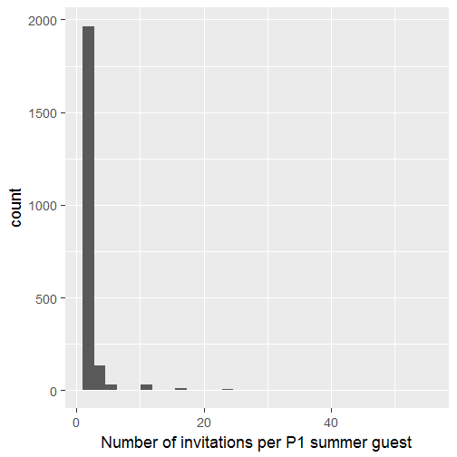
As I said earlier some guests were invited several times. I want to look at the distribution of the number of invitations per guest.
invites <- dplyr::select(sommargaester, name, rep)
invites <- dplyr::group_by(invites, name)
invites <- dplyr::summarize(invites, no_invites = max(rep))
invites <- unique(invites)
library("ggplot2")
 theme_set(theme_gray(base_size = 18))
ggplot(invites) +
  geom_histogram(aes(no_invites)) +
  xlab("Number of invitations per P1 summer guest")

Some people have been invited a lot! If you remember my initial tables, it had only a few columns for the episode dates but one guest could have several lines.
Who are the people that got invited that many times?
jobs <- dplyr::select(occupation, name, occupation)
jobs <- unique(jobs)
invites <- dplyr::left_join(invites, occupation, by = "name")
invites <- dplyr::select(invites, name, no_invites, occupation)
invites <- unique(invites)
invites <- dplyr::group_by(invites, name, no_invites)
invites <- dplyr::summarise(invites, occupation = toString(occupation))
invites <- dplyr::ungroup(invites)
invites <- dplyr::arrange(invites, desc(no_invites))
knitr::kable(invites[1:20,])
| name | no_invites | occupation |
|---|---|---|
| Torsten Ehrenmark | 54 | journalist, translator, writer |
| Jörgen Cederberg | 53 | NA |
| Gösta Knutsson | 42 | cartoonist, journalist, translator, children’s writer, writer |
| Maud Reuterswärd | 35 | writer |
| Georg Eliasson | 29 | screenwriter |
| Pekka Langer | 29 | television presenter, actor |
| Britt Edwall | 24 | writer |
| Arne Ericsson | 23 | musician |
| Bengt Feldreich | 23 | journalist, television presenter |
| Berndt Friberg | 23 | journalist |
| Carl-Olof Lång | 23 | director |
| Carl-Uno Sjöblom | 23 | television presenter |
| Lars Ulvenstam | 23 | journalist |
| Lars Widding | 23 | journalist, writer |
| Åke Falck | 17 | film director, director, television presenter, screenwriter, actor |
| Barbro Alving | 17 | journalist, screenwriter, writer |
| Bo Setterlind | 17 | writer, poet |
| Bo Strömstedt | 17 | NA |
| Elisabeth Söderström | 17 | singer, opera singer |
| Fredrik Burgman | 17 | journalist |
Most frequent occupations (by episode)
everything <- dplyr::group_by(occupation, occupation)
everything <- dplyr::summarize(everything, n = n())
everything <- dplyr::filter(everything, n > 50)
library("magrittr")
everything %>%
  dplyr::arrange(n) %>%
  dplyr::mutate(occupation = factor(occupation, ordered = TRUE, levels = unique(occupation))) %>%
ggplot() +
  geom_col(aes(occupation, n)) +
  theme(axis.text.x = element_text(angle = 90, hjust = 1)) +
  ggtitle("Number of episodes by occupation",
subtitle = "for occupations represented more than 50 times")

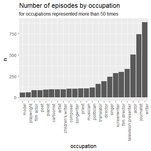
So in terms of episodes I’d say the media and culture fields are quite well represented. That said it might also be due to the fact that a person doing sports for instance will be classified as either ice skater or sprinter, so there’s no chance for sports to appear here. I’ll leave the classification of occupations in categories as an exercise for the reader though.
Most frequent occupations (by unique guest)
everything <- dplyr::select(occupation, name, occupation)
everything <- unique(everything)
everything <- dplyr::group_by(everything, occupation)
everything <- dplyr::summarize(everything, n = n())
everything <- dplyr::filter(everything, n > 20)
library("magrittr")
everything %>%
  dplyr::arrange(n) %>%
  dplyr::mutate(occupation = factor(occupation, ordered = TRUE, levels = unique(occupation))) %>%
ggplot() +
  geom_col(aes(occupation, n)) +
  theme(axis.text.x = element_text(angle = 90, hjust = 1)) +
  ggtitle("Number of guests by occupation",
subtitle = "for occupations represented more than 20 times")

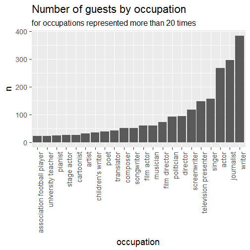
With this figure by guest rather than by episode, a bit more diversity has appeared, e.g. “university professor” and “association football player”. Moreover although this was a nice exercise I won’t pretend that someone’s occupation characterizes them fully! The P1 summer guest programm really presents a variety of episodes, and I’d tend to think everyone can find an episode that they appreciate. For instance I remember liking the baker Sébastien Boudet’s episode (yep he’s French) and the one featuring the former high jumper Kajsa Berqvist. Now all this data munging has left me more than ready to look at the list of episodes again to choose the next ones I’ll listen to!